WelcomeWhat this is, and who it is for
OpenSpineConsortium builds openly licensed datasets of the spine and pelvis and the tools to measure them. Our flagship, CTSpinoPelvic1K, is 802 abdominopelvic CT scans with every vertebra, the sacrum, the first sacral segment, both hip bones, both femora and every rib labeled on one coordinate frame, plus the anatomy that makes lumbar numbering ambiguous recorded as itself. Students built it. Students are now using it to answer anatomical questions at a scale a cadaver lab never reaches.
This primer is the on-ramp. It assumes nothing: not a terminal, not Python, not git. Each section ends with something concrete you can check. Work through it in order the first time; afterwards it is a reference.
What you will be able to do
Open a labeled CT, measure a bone across 802 people, compare groups, draw the figure, and hand in a study someone else can rerun.
How long it takes
One afternoon for the toolkit and the grid. One evening for the dataset and the demo. Your own project starts on day three.
How you get help
Claude Code, in your editor, for the code. The workshop tutorials for depth. Your mentor, by pull request and ClickUp, for the science.
Start here: one command. Make a Claude account and subscribe to Claude Pro (about $20 a month; it includes Claude Code, the assistant that will write and run your code), make a free GitHub account, then open a terminal and paste the line for your computer:
macOS / Linux / WSLTerminal
curl -fsSL https://openspineconsortium.com/onboard.sh | bash
WindowsPowerShell
irm https://openspineconsortium.com/onboard.ps1 | iex
It installs what is missing (Git, the GitHub CLI, VS Code with the Claude Code extension, Claude Code), clones the Student_Projects repository into ~/OpenSpineConsortium, and starts Claude on /onboard, which does Sections 1 to 6 with you one step at a time: GitHub and Hugging Face sign-in, the SSH key to the grid, the environment and the dataset on the grid, the demo study, and a project proposal. It stops only for the three things that need your university identity (the grid account request, the Google Authenticator scan, and one password-plus-code login), and tells you exactly what to do at each. Run the same line again any time; it resumes where you were. The rest of this page explains what it is doing and why, so you can do any step by hand.
Section 1The toolkit
Four installs. Each is a download and a click except Python, which comes from a terminal command the linked tutorial gives you verbatim.
1.1 An editor: Visual Studio Code
Download from code.visualstudio.com and install with the defaults. On the first launch install two extensions from the Extensions panel (Ctrl+Shift+X on Windows, Cmd+Shift+X on a Mac): Python (by Microsoft) and Remote - SSH (by Microsoft). Remote - SSH is how you will edit files on the grid as if they were on your laptop.
1.2 A command line and git
macOSXcode Command Line Tools
Open Terminal (Applications → Utilities) and run xcode-select --install. Accept the dialog. This installs git and the compilers Python packages need. You do not need the full Xcode app.
WindowsGit for Windows and WSL
Install Git for Windows with the defaults, which gives you Git Bash. Then, in an administrator PowerShell, run wsl --install and reboot: Windows Subsystem for Linux gives you the same Linux terminal the grid has, so every command in this primer works unchanged.
1.3 Python: Miniforge
Follow Workshop Tutorial 1, steps 1 and 2. It installs Miniforge (Python plus the mamba package manager) and creates an imaging environment. Do it on your laptop now; you will repeat the same two steps on the grid in Section 2, and Claude can do it for you there.
1.4 Claude Code
Claude Code is an AI programming assistant that runs in your terminal and inside VS Code. It reads your files, writes and edits code, runs commands with your permission, and explains what it did. It is how most of your code will get written, and the reason this primer can promise a study by the end.
macOS / Linux / WSLInstall
curl -fsSL https://claude.ai/install.sh | bash
Windows PowerShellInstall
irm https://claude.ai/install.ps1 | iex
Then, in VS Code, install the Claude Code extension from the Extensions panel. Open a terminal (Ctrl+`), type claude, and sign in when the browser opens. You need a Claude account with Claude Code access; ask your mentor which plan the lab uses before buying anything.
Check: in a VS Code terminal, git --version, mamba --version and claude --version each print a version. If one does not, ask Claude in the terminal that works: paste the error and say what you were installing.
Section 2The grid
The Wayne State grid is a Linux cluster with far more CPU, memory and GPU than your laptop, run by SLURM, a job scheduler. You log in to a small "login node" to edit files and submit jobs; the jobs run on the big nodes. The rule is simple: anything heavier than a minute of work runs as a job, never on the login node.
2.1 Get an account, and set up Google Authenticator
Accounts are tied to your WSU AccessID and sponsored by a faculty member. Request one through Wayne State C&IT's High Performance Computing pages at tech.wayne.edu/kb/high-performance-computing (the "Grid account request" form) and name Gregory Schwing as sponsor. Email him that you have applied so he can confirm it. Accounts are usually created within two business days; hpc@wayne.edu answers questions.
The grid's second factor is Google Authenticator, not the Microsoft Authenticator the rest of the university uses. Install the app on your phone, connect to the WSU VPN, log in to ondemand.grid.wayne.edu with your AccessID and password, open Interactive Apps → 2FA Setup, launch it, and scan the QR code with the app. From then on a password login to the grid asks for the six-digit code. C&IT's step-by-step article has screenshots.
2.2 Make an SSH key, so the code is asked only once
An SSH key is a pair of files: a private one that stays on your laptop and a public one you give to the grid. It lets you log in without a password or a phone code, and that matters here for a specific reason: Claude drives the grid with non-interactive ssh commands, which cannot answer a two-factor prompt. You type the password and the Authenticator code exactly once, to install the key. In your laptop terminal (Terminal, Git Bash, or WSL), or let /onboard run these for you:
# make the key; press Enter at every prompt, or add a passphrase you will remember
ssh-keygen -t ed25519 -C "youraccessid@wayne.edu"

# copy the public half to the grid (type your grid password once)
ssh-copy-id youraccessid@grid.wayne.edu

# from now on this logs you in without a password
ssh youraccessid@grid.wayne.edu
On Windows Git Bash, if ssh-copy-id is missing, do it by hand: cat ~/.ssh/id_ed25519.pub | ssh youraccessid@grid.wayne.edu "mkdir -p ~/.ssh && cat >> ~/.ssh/authorized_keys".
2.3 Give the grid a short name
Create or edit ~/.ssh/config on your laptop so that ssh grid is enough:
Host grid
    HostName grid.wayne.edu
    User youraccessid
    IdentityFile ~/.ssh/id_ed25519
2.4 Two ways to work, and the one we use
The lab's setup, and the one this primer assumes: Claude Code runs on your laptop, in VS Code, and drives the grid over SSH. Code moves through git (commit locally, push, pull on the grid), jobs are submitted with a short ssh grid "cd ~/Student_Projects && sbatch ...", a background loop polls the queue, and results come back with rsync. Your editor, your files and your assistant stay in one place; only the computing happens remotely. On Windows, Claude runs those network commands through WSL, which is why Section 1.2 installs it.
The alternative is to work on the grid directly: press F1, choose Remote-SSH: Connect to Host, pick grid, and a VS Code window opens whose files and terminal live there; install Claude Code on the grid with the Linux command from Section 1.4. This is fine for editing and for quick looks at data, but the login node is shared and small, so heavy work is still a SLURM job.
Both ways depend on the SSH key and the grid alias from 2.2 and 2.3. Test them now: ssh -o BatchMode=yes grid hostname must print warrior without asking for anything.
2.5 SLURM in five commands
| command | what it does |
|---|---|
sbatch job.sh | submit a job script; prints a job id |
squeue -u $USER | list your jobs and whether they are waiting or running |
scancel <jobid> | stop a job |
tail -f logs/<name>_<jobid>.out | watch a job's output as it runs |
sacct -j <jobid> --format=JobID,State,Elapsed,MaxRSS | after it ends, how long it took and how much memory it used |
Workshop Tutorial 5 walks through a job script line by line. The template job script in Student_Projects is the one you will actually use.
Where files live. Your home directory is small and backed up; put code and results there. Large data lives in the shared dataset folder your mentor names. Never put CT volumes in git, and never run a long script on the login node.
2.6 Three rules the lab learned the hard way
- Job scripts are files, never heredocs. Every attempt to push a script through
sshinline, or to pass a multi-part command throughsbatch --wrap, was mangled by quoting: variables expanded on the wrong machine, backslashes eaten, commands split. Write the job script into the repository, commit it, pull it on the grid, submit it there. - Anything longer than a minute is a batch job, even if it is light. The login node is shared, and an SSH session that runs long gets cut.
- Poll in the background. A job that takes twenty minutes is checked by a loop that asks
squeueevery thirty seconds and prints the log when the job is gone. Neither you nor Claude should sit in the foreground waiting.
These rules are written into the CLAUDE.md you will copy in Section 3, and into tools/grid.sh in Student_Projects, which wraps the five remote calls a project needs:
tools/grid.sh run "squeue -u \$USER"                       # a short command on the login node
tools/grid.sh sync                                          # git pull the grid clone
tools/grid.sh submit templates/slurm_job.sh projects/me/measure.py --data ~/data/CTSpinoPelvic1K --out projects/me/results
tools/grid.sh wait 40056610                                 # poll every 30 s, then print the logs
tools/grid.sh pull projects/me/results projects/me/results  # rsync a results folder back
Section 3Teaching Claude to work on the grid
The short path. Clone Student_Projects, open it in VS Code, type claude, then type /onboard. The repository's root CLAUDE.md gives Claude the whole lab workflow the moment it opens the folder, and /onboard walks you through everything in Sections 2 to 6: it checks your tools, makes the SSH key and installs it, builds the environment and fetches the dataset on the grid as jobs, runs the demo, and then helps you choose a project from projects/IDEAS.md and write the proposal. The only things it cannot do for you are the account request and the Authenticator scan. GETTING_STARTED.md is the one-page version.
Claude Code reads a file called CLAUDE.md at the start of every session: the one at the root of Student_Projects for the lab as a whole, and the one in your project folder for your project. That file is where you tell it, once, how the grid works, where the data is, and which rules never bend. Student_Projects ships a template; /new-project copies it into your project folder and fills in the three lines marked EDIT.
With that in place, these are the prompts that do the work. Type them to Claude in the VS Code terminal on the grid.
Create the mamba environment from templates/environment.yml in my home
directory and show me how to activate it.

Write a SLURM job script from templates/slurm_job.sh that runs
projects/<me>/measure_something.py with 8 workers and 32 GB of memory.
Do not submit it; show it to me and explain each #SBATCH line.

My job 123456 failed. Here is the tail of logs/osc_measure_123456.err:
<paste>   What went wrong and what do I change?
Two habits keep you in charge. Claude drafts, you submit: read the job script, then run sbatch yourself, or say "submit it" and let Claude run exactly the one command. Claude explains, you decide: when it proposes a measurement, ask it which label identifiers it is using and why, and check them against dataset_labels.json. The template CLAUDE.md already tells it to work this way.
3.1 What the template CLAUDE.md carries
It is the lab's working knowledge written down, so that a new project starts where the last one left off rather than from zero:
- the two machines and how they talk (laptop, WSL on Windows, the
gridalias, the login nodewarrior, where the repository and the data live on each); - the seven rules that never bend (login node, scripts as files, Claude drafts and you submit, never reorient a volume, never assume an axis, never commit data, never edit a result by hand);
- the remote workflow step by step, from commit to
rsync, with the exact commands; - SLURM defaults for this grid: the
primaryandgpuqueues, the H200 GPU request, memory and time to ask for, node-local scratch, how long an 802-record pass takes; - the laptop pitfalls that cost afternoons (heredoc backslashes, files locked by a viewer, spaces in OneDrive paths, PowerShell without
&&); - how you want to work (one script per output, ten records before 802, a journal line per decision) and what Claude should do at the start of every session.
3.2 Slash commands and permissions
Student_Projects also ships a .claude/ folder that Claude Code reads automatically from the repository:
| command | what it does |
|---|---|
/onboard | the whole setup, resumable: tools, SSH key, grid clone, environment and dataset as jobs, the demo, then a project from the ideas list |
/grid-status | checks the grid answers, lists your jobs, shows the last job's log tail |
/grid-submit <what> | writes the job script as a file, commits, syncs the grid, shows you the submit command, waits for your word, then submits and starts the background wait |
/grid-pull <folder> | rsyncs a results folder back, opens every figure, checks a report number against its CSV |
/new-project <topic> | creates your project folder and branch, then interviews you section by section to write the proposal |
.claude/settings.json sets the default mode to accept file edits automatically and pre-approves the routine commands (git, python, ssh to grid, rsync, the GitHub and Hugging Face tools, the helper script) so you are not asked to confirm each one, and forbids the destructive ones (force-push, hard reset, deleting a repository). It lives in git, so the whole lab shares the same defaults. When Claude does ask about something outside that list, "Yes, and don't ask again" makes the answer permanent for the repository. If you would rather never be asked on your own laptop, /onboard offers at the start to set bypassPermissions in your user settings and explains what that means; the deny list still applies and /permissions turns it back.
Check: from your project folder on the grid, claude starts, and asking "what does CLAUDE.md say I should never do?" gets back the rules about reorienting volumes, assuming axes, and committing data.
Section 4The dataset: CTSpinoPelvic1K
802 abdominopelvic CT scans from one prospective screening trial (ACRIN 6664, 15 centers, five scanner vendors), each with a label volume on the same grid as the image. A label volume is an image whose voxels hold integers naming the structure at that point. The integers are the label scheme.
4.1 The label scheme (v10)
The authoritative list is dataset_labels.json in the download. Read it in code; do not type identifiers from memory.
4.2 The manifest
manifest.json has one row per record. The fields you will group by most: sex (female 393, male 345, other 11, missing 53), age (709 records), position (prone or supine), castellvi_type (33 records; null means ungraded, not normal), has_l6, has_lumbar_rib, n_lumbar_labels, hardware_labelled, plus scanner make, model, kernel and slice thickness.
4.3 Four rules before any analysis
They are in KNOWN_ISSUES.md, which ships with the data. Read the whole file once; these four bite most often.
- A null Castellvi grade means nobody looked. Do not count it as normal.
- Exclude the 11 hardware records from anything measured across a joint or a gap; eight of them have replaced hips.
- Do not pool prone and supine for anything postural (lordosis, sacral slope, pelvic tilt). Widths are fine.
- Nine four-lumbar records carry the fused transitional vertebra under the S1 identifier. Filter on
n_lumbar_labelsif that matters to you.
4.4 Get the data
The labels and metadata are 1.1 GB. The CT images are another 195 GB; download them only when you need voxel intensities (bone density, Hounsfield units), and on the grid, not your laptop.
# in your mamba environment
python - <<'EOF'
from huggingface_hub import snapshot_download
snapshot_download("OpenSpineConsortium/CTSpinoPelvic1K", repo_type="dataset",
                  local_dir="CTSpinoPelvic1K",
                  allow_patterns=["labels/*", "manifest.json", "dataset_labels.json",
                                  "KNOWN_ISSUES.md", "splits_5fold.json", "README.md"])
# add "ct/*" to allow_patterns for the images (195 GB)
EOF
The archival copy is on Zenodo, 10.5281/zenodo.22642578, which is what you cite. On the grid, ask your mentor for the path of the shared copy rather than downloading your own.
4.5 Look at it
Before measuring anything, look at a record. Install ITK-SNAP, open ct/0007_ct.nii.gz as the main image and labels/0007_label.nii.gz as a segmentation, and load the label descriptions from the descriptor script so the colors have names. Workshop Tutorial 4 covers the viewer; Tutorial 2 explains the file format.
Section 5The demo study: is the female pelvis relatively wider?
Every project here has the same shape: a question, a measurement made from labels, a comparison between groups, a figure, and a report whose numbers come from a file the script wrote. The demo does all five in one 120-line script you can read in ten minutes. It lives in examples/pelvic_width_dimorphism/ of Student_Projects.
5.1 The question and the measurement
Is the pelvis wider in females, once you allow for the size of the skeleton it sits on? The textbook dimorphism is a wider hip joint separation relative to skeletal size, so that is what the script measures. Each femoral head centre is the centroid of the medial-most 28 mm of the top 30 mm of the femur label (identifiers 32 and 33); the distance between the two centres is the femoral head distance. The skeletal reference is the left–right width of the anterior 18 mm of the L4 body (23). Their ratio is the number the question is about. The script also walks the line through the two head centres outward to where it leaves each femur mask, giving the outer width on the same axis, and records the plain bi-iliac width of the hip bones (30, 31) for comparison. Every axis is read from the file's affine, so prone and supine records are measured identically.
5.2 Run it
git clone https://github.com/OpenSpineConsortium/Student_Projects.git
cd Student_Projects
mamba activate osc
python examples/pelvic_width_dimorphism/measure_pelvic_width.py \
    --data /path/to/CTSpinoPelvic1K --out examples/pelvic_width_dimorphism/results --workers 8
About an hour on eight laptop CPUs, because every record is a full label volume; add --from-csv to rebuild the report and figure from a finished CSV in seconds. On the grid, wrap the same command in templates/slurm_job.sh and sbatch it.
5.3 What it finds
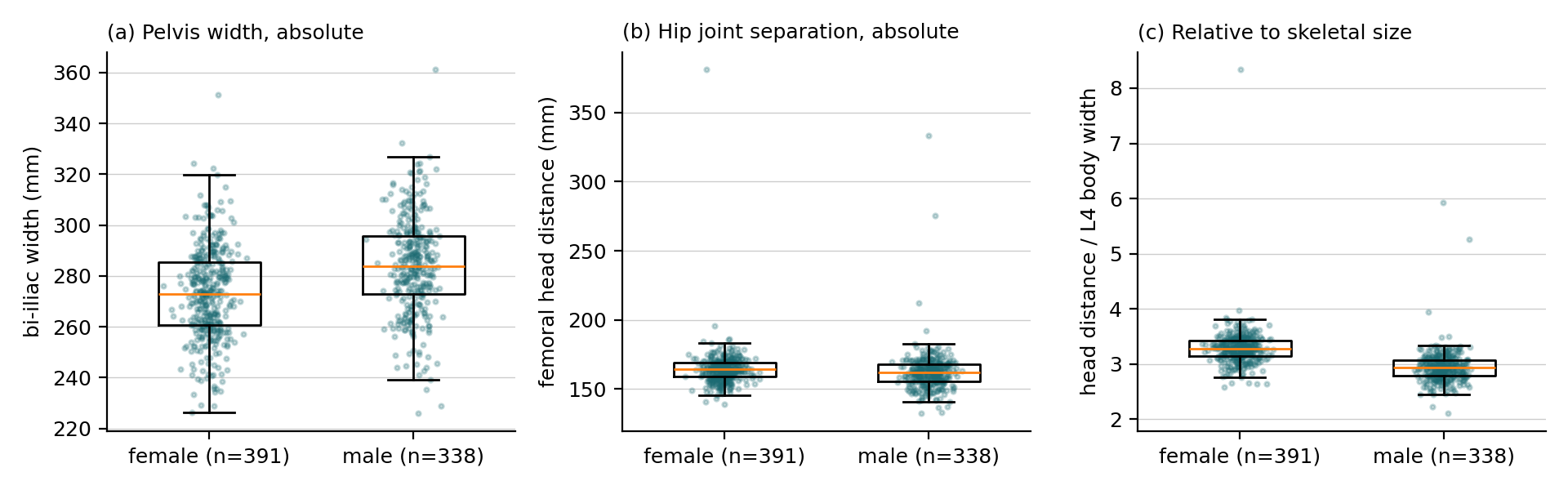
The answer is yes, and the three panels tell it in order. Male pelves are wider at the iliac crests in absolute terms (a). The femoral heads sit the same distance apart in both sexes, about 163 mm (b). Male skeletons are bigger, so the same joint separation on a smaller skeleton is a relatively wider pelvis: divided by L4 body width the ratio is 3.29 in females against 2.94 in males (391 females, 338 males), a large effect that separates the two distributions at a glance (c). The published value of this ratio is 3.95 against 3.48; ours is lower because a label-derived body width runs a few millimetres wider than a caliper endplate width, and it is the female to male ratio, 1.12 against 1.14, that agrees. Two lessons sit in this run. The first measurement we tried, bi-iliac width over S1 width, answered "no" with a small effect; the measurement decides which question you actually asked. And the far outliers in (b) and (c) are records where a femoral head was not where the label said (a fragment or a prosthesis); the medians do not move, but an honest report says they are there. Every number above is in results/report.txt, written by the script from results/pelvic_width.csv, one row per record. That is the standard for your project too: if a number appears in your text, a script wrote it to a file first.
5.4 Make it yours
Change one thing at a time. Divide by S1 width (identifier 29) instead of L4 and you have a sacral reference. Use the outer width instead of the head distance and you have the acetabular span. Group by position instead of sex and you test whether posture changes a distance (it should not; that is a useful sanity check). Group by has_l6 and you have a transitional-anatomy question. Ask Claude to make the change and to explain the two lines it edited.
Section 6Your project
Two repositories, one folder. Student_Projects is public and holds the tools, templates, the demo, the ideas list and this onboarding. Projects is private and holds the projects themselves, one folder each; it is cloned inside the public one as projects/. Proposals are reviewed as pull requests in the private repository, so only collaborators see them and your idea stays yours until it is published. Approved projects are tracked in ClickUp.
6.1 Get access
Make a free GitHub account if you do not have one, then email your GitHub username to gregory.schwing@med.wayne.edu with the subject "Projects access". You will be added as a collaborator on the private repository; /onboard clones it into place once you are.
6.2 Choose a question, then write the proposal
If you do not arrive with a question, projects/IDEAS.md holds about twenty, drawn from the dataset paper's future directions, the site gallery's cases, and the lab's open tasks, each written the way a proposal has to state it: the measurement with its identifiers, axis and unit, the comparison, a difficulty from one to three, and the source. /onboard ends by asking three questions and proposing three of them that fit you.
Copy templates/proposal_template.md to projects/<lastname>_<topic>/proposal.md and fill in every section: the question, what is known, exactly what you will measure (identifiers, axis, unit), who you compare and what you exclude, the analysis, the outputs, milestones with dates, and what could go wrong. One page. The worked example, schwing_pelvic_width_dimorphism, is the demo study written as a proposal; imitate it.
6.3 Open the pull request
/new-project <topic> does all of this with you and opens the pull request at the end. By hand, every command runs inside projects/, the private repository:
cd projects
git checkout -b proposal/<lastname>-<topic>
mkdir -p <lastname>_<topic>
cp ../templates/proposal_template.md <lastname>_<topic>/proposal.md
# ... edit the proposal ...
git add <lastname>_<topic>/proposal.md
git commit -m "Proposal: <title>"
git push -u origin proposal/<lastname>-<topic>
gh pr create --fill --base main
The PR template asks for the email address that should receive your ClickUp invitation, the mentor you are requesting, and a checklist (onboarding done, demo run, no data files). Fill all of it. The example proposal shows what a complete one looks like.
6.4 Review, approval, ClickUp
Your mentor reviews in the PR thread; expect questions about the measurement and the exclusions, and revise by pushing to the same branch. When the proposal is approved the PR is merged and a ClickUp invitation goes to the email you gave. Your milestones become tasks there; that is where progress, blockers and deadlines are tracked from then on. Code and results keep going into your project folder by pull request, each one naming its ClickUp task.
6.5 Working with your mentor
- One branch per piece of work, a pull request when it is ready for eyes, never a commit straight to
main. - Keep
JOURNAL.mdin your folder: a dated line whenever something worked or failed. It becomes your methods section. - Every figure has a script that makes it; every number in your text was written to a file by that script.
- Ask early. A question in the PR thread or a ClickUp comment costs nothing; a week lost to a wrong identifier costs a week.
- Authorship follows the ICMJE criteria and is settled by contribution, recorded as you go.
Section 7Basics you will need
7.1 The terminal in ten commands
| command | meaning |
|---|---|
pwd | where am I |
ls -la | what is here |
cd folder · cd .. | go into a folder · go up one |
mkdir -p a/b | make folders |
cp src dst · mv src dst · rm file | copy · move or rename · delete (no undo) |
cat file · head file · tail -f file | print a file · its first lines · follow it as it grows |
grep -n word file | find lines containing a word |
python script.py --help | run a script; every script here explains its options |
| Ctrl+C | stop what is running |
| Tab | autocomplete a file name; press it constantly |
7.2 Git in six commands
git clone <url>          # copy a repository to your machine
git checkout -b name     # start a branch for a piece of work
git status               # what changed
git add file             # stage a change
git commit -m "what"     # record it, with a message that says what and why
git push -u origin name  # send the branch to GitHub; then open a pull request there
7.3 Reading a label volume in twenty lines
import json, numpy as np, nibabel as nib

img = nib.load("CTSpinoPelvic1K/labels/0007_label.nii.gz")
lab = np.asanyarray(img.dataobj)                 # the integer volume; never reorient it
names = json.load(open("CTSpinoPelvic1K/dataset_labels.json"))["id_to_name"]

ids, counts = np.unique(lab, return_counts=True)
for i, n in zip(ids, counts):
    print(i, names[str(i)], n, "voxels")

codes = nib.aff2axcodes(img.affine)              # which array axis is left-right?
lr = [k for k, c in enumerate(codes) if c in "LR"][0]
mm = img.header.get_zooms()[lr]                  # voxel size along it
hips = np.isin(lab, [30, 31])
cols = np.nonzero(hips.any(axis=tuple(k for k in range(3) if k != lr)))[0]
print("bi-iliac width:", (cols.max() - cols.min() + 1) * mm, "mm")
7.4 The manifest in five lines
import pandas as pd
m = pd.read_json("CTSpinoPelvic1K/manifest.json")
print(m["sex"].value_counts(dropna=False))
print(m.groupby("sex")["age"].describe())
print(m[m["has_l6"]][["label_file", "castellvi_type", "n_lumbar_labels"]])
7.5 Asking Claude well
- Say what you want to end up with, not how: "a CSV with one row per record and the width in mm" beats "loop over the files".
- Give it the facts it cannot see: paste the error, the log tail, the identifier list.
- Ask it to explain before it edits: "which lines will you change, and why?"
- Ask for small steps: ten records first, then all 802.
- When it is confident and you are not, ask it to check: "print the unique identifiers in that volume and confirm 29 is present."
7.6 Reproducibility, the short version
- The environment is a file (
environment.yml), and the file is in git. - One script per output, run from the repository root, with its options in
--help. - Random things get a seed. Figures get a caption in the script's docstring.
- Results are written by scripts, never edited by hand; if a number is wrong, fix the script and rerun.
- Cite the dataset by DOI, and say which version.
The workshop tutorials go deeper: running a pretrained segmentation network, training one on the grid, and writing the paper.
Section 8You are onboarded when
- VS Code, git, mamba and Claude Code all answer
--versionon your laptop. ssh gridlogs you in without a password, and VS Code opens your grid home folder.- Claude Code on the grid can recite the rules in your CLAUDE.md.
- The labels and manifest of CTSpinoPelvic1K are on disk, and you have opened one record in ITK-SNAP.
- The demo study ran end to end and its report matches the numbers in Section 5.
- Your proposal is a pull request in Student_Projects, with the email for your ClickUp invitation filled in.
Then the science starts. Welcome.